In this page
This page explains how to process GAOES-RV data with IRAF reduction package as general high-dispersion spectra whose R is ∼ 65,000.
| In addition to the general high-dispersion spectral analysis described in this page, special analysis is required when performing precise radial velocity measurements using the I2 cell. If you expect it, we strongly recommend that you contact the PI (Bun'ei Sato, Tokyo Institute of Technology, satobn__at__eps.sci.titech.ac.jp) and conduct joint research. |
For QL in the Seimei telescope observation environment, start from this procedure (Make Flat).
Spectral Format
| Aperture | Echelle Order | Wavelength [Å] | Note |
|---|---|---|---|
| 1 | 101 | 5857.40 — 5952.46 (5920) | long side cut by the chip edge |
| 2 | 102 | 5799.96 — 5894.13 | |
| 3 | 103 | 5743.63 — 5836.93 | partially damaged by bad column |
| 4 | 104 | 5688.39 — 5780.82 | |
| 5 | 105 | 5634.20 — 5725.78 | |
| 6 | 106 | 5581.04 — 5671.78 | |
| 7 | 107 | 5528.04 — 5619.43 | |
| 8 | 108 | 5477.67 — 5566.77 | |
| 9 | 109 | 5427.40 — 5515.71 | |
| 10 | 110 | 5378.06 — 5465.58 | |
| 11 | 111 | 5329.60 — 5416.35 | |
| 12 | 112 | 5282.01 — 5368.00 | |
| 13 | 113 | 5235.25 — 5320.50 | |
| 14 | 114 | 5189.32 — 5273.84 | |
| 15 | 115 | 5144.19 (5198) — 5227.98 | short side cut by the chip edge |
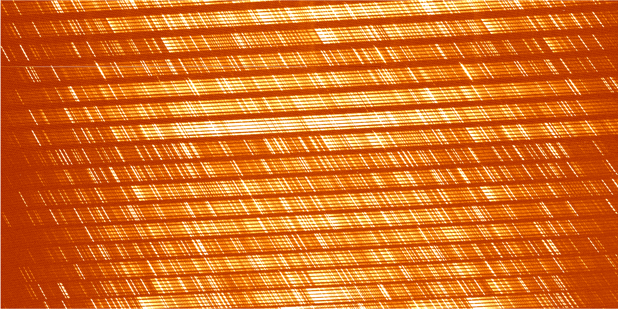
The slit length direction of the GAOES-RV spectrum is not parallel to the line of CCD pixels.
Therefore, it is necessary to add up after performing wavelength calibration
by tracing one pixel at a time in the dispersion direction.
This process can be done by using the following IRAF cl-scripts.
IRAF CL-script download and preparation
Download script package
All scripts useed in this page can be download via the following github page.
https://github.com/chimari/hds_iraf
The scripts are involved in the reduction package for Subaru/HDS.
The gaoes package has been confirmed to work with IRAF v2.16.2, V2.17, and PyRAF environment.
Install the entire of hds_iraf package.
- Just download all files of hds_iraf packages, then add
set    hdshome = 'home$IRAF/hds_iraf/'
task   $hds.pkg = 'hdshome$hds.cl'
set    gaoeshome = 'home$IRAF/hds_iraf/'
task   $gaoes.pkg = 'gaoeshome$gaoes.cl'
in your login.cl .
* Please change ''home$IRAF/hds_iraf/'' to the directory in which you put your hds_iraf package. - Load gaoes packages after started the IRAF shell.
ecl> gaoes *************************************************************** *************************************************************** ** Seimei GAOES-RV IRAF Reduction Package ** ************************** CAUTION !!! ************************ ** This package is always under development. ** ** Check the latest package via ** ** git clone https://github.com/chimari/hds_iraf ** ** ** ** This package is developed by Akito Tajitsu (NAOJ) ** ** last update : 2023/03/27 ** *************************************************************** *************************************************************** gaoes_comp gaoes_linear gaoes_overscan mkblaze wacosm11 gaoes_ecfw gaoes_linstab grql sed wacosm3 gaoes_flat gaoes_linstat hdsmk1d wacosm1 gaoes> - Please see here for more details about HDS IRAF package.
GAOES-RV reference download
Please download from here.
http://www.o.kwasan.kyoto-u.ac.jp/inst/gaoes-rv/GAOES-RV_ql-20240926.tar.gz
The archive file includes reference frames and databace files (aperture, flat, comparison, mask, and blaze function) and python scripts for QL application (grlog).
Extract the archive and put the "GAOES-RV_ql/" directory into an appropriate place (HOME$/IRAF/GAOES-RV_ql/ is the default for grlog).
Reduction
Start
- You need to create a new your working directory.
- Copy reference and database files in ''GAOES-RV_ql-XXXXXXXX.tar.gz'' into your working directory.
- The current file tree of your working directory should be
work
├── Ap.GAOES-RV.f8(fc).fits
├── ThAr.GAOES-RV.f8(fc).center.fits
├── Mask.GAOES-RV.ocs_ecfw.fits
├── cBlaze.GAOES-RV.f8(fc).fits
└── database
    ├── apAp.GAOES-RV.f8(fc)
    └── ecThAr.GAOES-RV.f8(fc).center
"f8" is for the octagon fiber and "fc" is for the circular fiber.
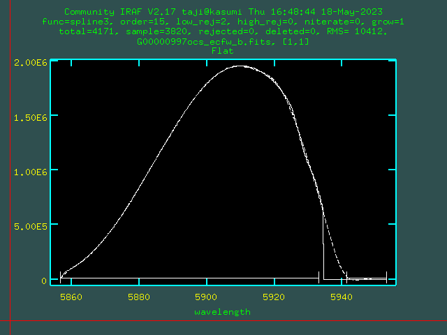
making Flat
- Make a list of flat frames, in which involves 8 digits of raw GRA fits files.
00000299
00000300
00000301
00000302
00000303
00000304
00000305
00000306
00000307
00000308
00000309
00000310
00000311
00000312
00000313
You can easily create the file using this commandseq -f "%08g" 299 313 > flat.in
- Use the task ''gaose_flat''.
PACKAGE = hds
   TASK = gaoes_flat

inlist  =              flat.in  input flat image list
indirec = /home/taji/work4/20221015  directory of RAW data
outimg  =         Flat20221015  output flat image

(ref_ap =       Ap.GAOES-RV.f8) Aperture reference image
(apflag =                  yes) Create new aperture reference? (yes/no)
(new_ap =           Ap20221015) New aperture image

(st_x   =                  -54) Start pixel to extract
(ed_x   =                   53) End pixel to extract

(scatter=                  yes) apscatter? (yes/no)
(normali=                  yes) apnormalize? (yes/no)

(mode   =                    q)
- inlist : created list file
- indirec : directory name of raw data
- outimage : flat file name to be created (add ''.ac'' for apscattered, and ''.nm'' for apnormalized to this file name)
- ref_ap : aperture reference (should be ''Ap.GAOES-RV''
- apflag : create a new aperture reference from the created flat image (''yes'' in usual)
- new_ap : new aperture reference image to be created
- st_x : minimum aperture for flat (∼ -54 in usual)
- ed_x : maximum aperture for flat (∼ 53 in usual)
- scatter : apscatter ? (''yes'' in usual)
- normalize : apnormalize ? (''yes'' in usual)
- The task ''gaoes_flat'' with the above parameter creates these files.
- Flat20221015.fits (imcombined flat)
- Flat20221015.sc.fits (scattered light subtracted flat by apscatter)
- Flat20221015.sc.nm.fits (normalized by apnormalize) ⇒ Input 2 for ''grql''
- Ap20221015.fits (aperture reference) ⇒ Input 1 for ''grql''
- database/apAp20221015 (aperture table)
making Comparison
- Use the task ''gaose_comp''.
- inid : 8 digit of ThAr GRA frame
- indirec : the directory where raw data are stored
- outimg : comparison frame name to be created
- ref_ap : aperture reference frame (created by ''gaoes_flat'')
- ref_com : wavelength calibrated reference (downloaded ''ThAr.GAOES-RV.center'' in usual)
- gaoes_comp with the above parameters creates these files.
- ThAr20221015.fits (overscanned 2D comparison image) ⇒ Input 4 for ''grql''
- ThAr20221015.center.fits (1D comparison spectrum traced the center 1 px of the 2D comparison image) ⇒ Input 3 for ''grql''
- database/ecThAr20221015.center (the wavelength table of the 1D spectrum)
PACKAGE = hds
   TASK = gaoes_comp

inid    =             00000315  input ID of ThAr frame
indirec = /home/taji/work4/20221015  directory of RAW data
outimg  =         ThAr20221015  output comparison image

(ref_ap =           Ap20221015) Aperture reference image
(ref_com= ThAr.GAOES-RV.f8.center) Wavelength reference (1D comparison) image

(mode   =                    q)
Object frame reduction
- Using flat and comparison frames made by the above procedures, reduce each object frame with the task ''grql''.
PACKAGE = gaoes TASK = grql inid = 00000944 Input frame ID (indirec= ..) directory of RAW data (batch = no) Batch Mode? (inlist = ) Input file list for batch-mode (interac= yes) Run task interactively? (yes/no) (ref_ap = Ap.GAOES-RV.fc) Aperture reference image (flatimg= Flat.GAOES-RV.fc.sc.nm) ApNormalized flat image (thar1d = ThAr.GAOES-RV.fc.center) 1D wavelength-calibrated ThAr image (thar2d = ThAr.GAOES-RV.fc) 2D ThAr image (st_x = -54) Start pixel to extract (ed_x = 53) End pixel to extract (cosmicr= yes) Cosmic Ray Rejection? (scatter= yes) Scattered Light Subtraction? (ecfw = yes) Extract / Flat-fielding / Wavelength calib.? (getcnt = yes) Measure spectrum count? (mk1d = no) Make order combined 1d spectrum? (splot = yes) Splot Spectrum? ### Cosmic-Ray Rejection. ### (cr_proc= wacosm) CR rejection procedure (wacosm|lacos)? ### Parameters for wacosm11 ### (cr_wbas= 2000.) Baseline for wacosm11 ### Parameters for lacos_spec ### (cr_ldis= no) Confirm w/Display? (need DS9) (cr_lgai= 1.67) gain (electron/ADU) (cr_lrea= 4.4) read noise (electrons) (cr_lxor= 9) order of object fit (0=no fit) (cr_lyor= 3) order of sky line fit (0=no fit) (cr_lcli= 10.) detection limit for cosmic rays(sigma) (cr_lfra= 3.) fractional detection limit fro neighbouring pix (cr_lobj= 5.) contrast limit between CR and underlying object (cr_lnit= 4) maximum number of iterations ### Scattered-light Subtraction ### (sc_inte= yes) Run apscatter interactively? ### Get Spectrum Count. ### (ge_line= 2) Order line to get count (ge_stx = 2150) Start pixel to get count (ge_edx = 2400) End pixel to get count (ge_low = 1.) Low rejection in sigma of fit (ge_high= 0.) High rejection in sigma of fit ### Make 1D spectrum ### (m1_blaz= ) Blaze Function (m1_mask= ) Mask Image (m1_stx = 60) Start X for trimming (m1_edx = 4120) Endt X for trimming ### Splot ### (sp_line= 1) Splot image line/aperture to plot (clean = yes) Clean up intermediate images? (yes/no) (mode = q)- inid : 8 digit of Object GRA frame
- indirec : the directory where raw data are stored
- batch : yes / no for batch mode (see below)
- inlist : input file list for batch mode
- ref_ap: Aperture reference image ⇐ Input 1 produced by ''gaoes_flat''
- flatimg: Normalized flat image ⇐ Input 2 produced by ''gaoes_flat''
- thar1d: 1D comparison spectrum ⇐ Input 3 produced by ''gaoes_comp''
- thar2d: 2D comparison image ⇐ Input 4 produced by ''gaoes_comp''
- st_x: minimum aperture for object frame. (should be the same value used in ''gaoes_flat'' ,∼ -54 in usual)
- ed_x: maximum aperture for object frame. (should be the same value used in ''gaoes_flat'' ,∼ 53 in usual)
- cosmicr: Do or skip Cosmic ray removal.
- scatter: Do or skip Scattered light subtraction.
- ecfw: Do or skip Extract / Flat-fielding / Wavelength calibration.
- getcnt: Automatic Count measurement.
- mk1d: Make complete 1D spectrum using blaze function.
- splot: Do or skip plotting the resultant spectrum.
- cr_proc: Cosmic Ray removal procedure (wacosm / lacos)
- cr_wbas: Baseline of wacosm11.
- cr_l*: parameters for lacos (You need to install STSDASS to use lacos_spec).
- sc_inte: Run apscatter interactively? (yes/no)
- ge_line: Echelle order line for automatic count measurement
- ge_stx: Start pixel in Echelle order for automatic count measurement
- ge_edx: End pixel in Echelle order for automatic count measurement
- m1_blaz: Blaze function for make 1D spectrum
- m1_mask: Mask image for make 1D spectrum
- m1_stx: Start pixel for scombine
- m1_edx: End pixel for scombine
- sp_line: Order number for splot
- With the above parameters, grql produces these files.
- G00000266o.fits (overscanned image)
- G00000266oc.fits (after cosmic ray removed)
- G00000266ocs.fits (after scatterd light subtracted)
- G00000266ocs_ecfw.fits (extracted + flat-fielded + wavelength calibrated spectrum) = filnal resultant
- G00000266ocs_ecfw_1d.fits (full 1D spectrum) = filnal resultant
- If you want to run grql for 2 or more object frames, you can use batch mode.
Create a list file, in which 8 digit numbers of GRA are stored.
00000321
00000322
00000323
00000324
00000325
...
Then, run grql with ''batch=yes'' and inlist=(object list file). - If you want to run grql in command line of ecl, the 8 digit number of object GRA must be enclosed in double quotations.
ecl> grql "00000321"
Make Full 1D spectrum
We have now obtained a multi-order echelle spectrum.
From now on, as an option, we will explain how to create a complete one-dimensional spectrum by connecting orders.
Make Mask
- Analyze one flat frame with grql in the same way as an object frame, and create G?????????ocs_ecfw.fits. (Until this point, set mk1d=no in grql)
- Use the task "gaoes_mkmask"
PACKAGE = gaoes
TASK = gaoes_mkmask

inimage =    G00000997ocs_ecfw  Input Flat image
mask    =        Mask.00000977  New Mask image

(mode   =                    q)
On each order when run, you will be asked as>>> Do you want to correct this order? (y/n) :
. Enter "y" if there is a bad pixel or an order edge and you want to correct it.
If you enter y, each order will be plotted, so move the cursor to one end of the range (X direction) you want to erase and press the "a" key.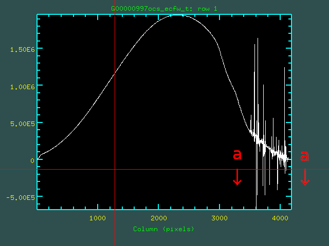
>>> Do you want to correct this order MORE? (y/n) :
answer "n" to proceed to the next order.
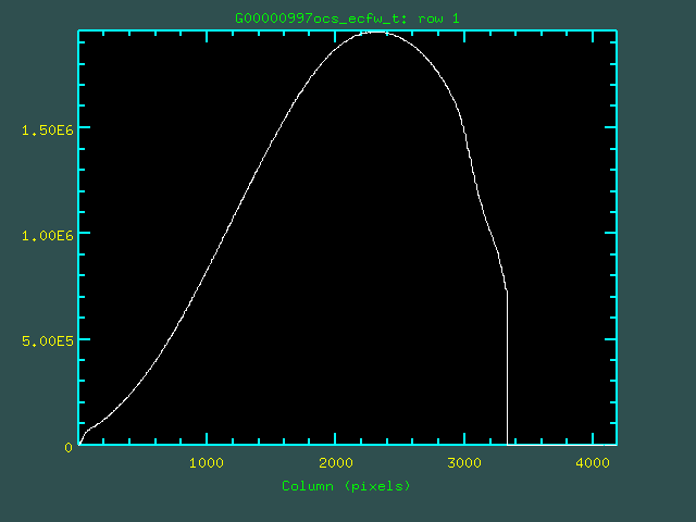
Repeating this for 15 orders creates a mask that eliminates unwanted areas.
Basically what you need to remove is only- Order of both ends (Order 1, 15)
- Order 3, Bad pixel around 5790A
Make Blaze function
Here we show how to do a continuous light fit to a flat spectrum and create a blaze function.
- For the input, use G????????ocs_ecfw.fits, which was analyzed with grql in the same way as the celestial object, using a flat sheet that was used to create the mask.
- Use the task "gaoes_mkblaze". Specify the mask frame created above in "mask".
PACKAGE = gaoes
   TASK = gaoes_mkblaze

inec    =    G00000997ocs_ecfw  Input Multi-Order Flat Spectrum
outblz  =      cBlaze.00000997  Output Blaze Function
(mask   =        Mask.00000997) Mask Image
(mode   =                    q)
When executed, the continuum task will be launched, so specify only the necessary parts in the spectrum with the "t" key, excluding the order end and badpixel,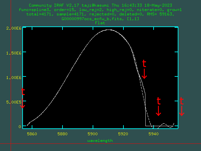
Repeating this for all 15 orders creates a blaze function.Key Description s Only use data between s and s. t Clear the area selected by s-key. f Fit the continuum curve. :order <number> Change fitting order (10-20 in usual). :niterate <number> Change fitting iteration number (0 in usual).
Basically, you need to be careful about the same parts on a multi-order spectrum as when creating a mask.
Make Full 1D object spectrum
Perform full one-dimensionalization of multi-order object spectra using the mask and blaze function created above.
- It is assumed that an echelle multi-order spectrum for an object frame (G??????????ocs_ecfw.fits) has been already created by grql.
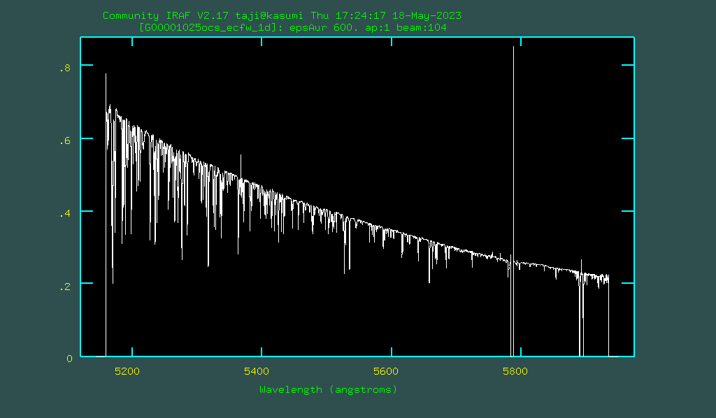
- Use the task "gaoes_mk1d".
PACKAGE = gaoes
   TASK = gaoes_mk1d

inec    =    G00001025ocs_ecfw  Input Multi-Order Spectrum
out1d   = G00001025ocs_ecfw_1d  Output 1D Spectrum
blaze   =      cBlaze.00000997  Blaze Function

(mask   =        Mask.00000997) Mask Image

(st_x   =                   70) Start X
(ed_x   =                 4100) End X

(mode   =                    q)
Specify the created files for "mask" and "blaze" respectively.
"st_x" and "ed_x" are numbers that specify in pixels from where to where to use for each order of the multi-order spectrum. Since the spatial direction of the spectrum is oblique in GAOES-RV, it is better to set the number with some leeway as specified above. It's a good idea to plot each order on splot, showing pixel scale on the horizontal axis with "$", and check roughly where the order edges are bent.
- When executed, a full 1D spectrum is automatically generated.
- Perform continuum fitting to the output full one-dimensional spectrum.
- Perform sensitivity correction using standard star data.
Make Full 1D spectrum by grql
Once you have created a mask and blaze function using flat data, you can use grql to create a full 1D spectrum from a raw data.
- Specify the parameters used by gaoes_mk1d such as "mask" and "blaze" with mk1d=yes in grql parameters.
PACKAGE = gaoes TASK = grql (...) (mk1d = yes) Make order combined 1d spectrum? (...) ### Make 1D spectrum ### (m1_blaz= cBlaze.GAOES-RV.f8) Blaze Function (m1_mask= Mask.GAOES-RV.f8.ocsf_ecfw) Mask Image (m1_stx = 60) Start X for trimming (m1_edx = 4120) Endt X for trimming - The out put will be G????????ocs_ecfw_1d.fits .
Conversion to heliocentric wavelength
The wavelengths analyzed so far are topocentric wavelengths.
By using the task rvgaoes, it is possible to convert to heliocentric wavelength that removes the influence of the rotation and revolution of the earth.
PACKAGE = gaoes
   TASK = rvgaoes

inimage =     SN2023ixf_Fcalib  Input image
outimage=  SN2023ixf_Fcalib.rv  Output image

(observa=               seimei) Observatory
(mode   =                    q)
login.cl に gaoesパッケージ中の obsdb.datを指定しておくと、observatoryとしてseimeiを選択することができます。 login.cl に gaoesパッケージ中の obsdb.datを指定しておくと、observatoryとしてseimeiを選択することができます。 Roguin. Cl ni gaoes pakkēji-chū no obsdb. Datto o shitei shite okuto, observatory to shite seimei o sentaku suru koto ga dekimasu. 75 / 5,000 翻訳結果 翻訳の結果 If you specify obsdb.dat in the gaoes package in login.cl, you can select seimei as an observer.
This task can be used for both multi-order and full 1D spectra.
Data Reduction on GUI (Quick Look)
Using the GUI "grlog" used in the observation environment of GAOES-RV, the same data analysis can be performed in each user′s environment.
The output spectrum is the same as the above grql executed on IRAF.
The Echelle multi-order spectrum is G??????????ocs_ecfw.fits, and the full one-dimensional spectrum is G????????ocs_ecfw_1d.fits.
- Requirements
- Linux environment where Gtk+3 can be used. (It has not been confirmed on Mac OS)
- Environment where PyRAF can be used.
- Preparation for PyRAF environment
PyRAF can be installed via astroconda/miniconda, and in Ubuntu it can be installed easily viasudo apt-get install astro-iraf python3-pyraf
Make sure that pyraf can be started from the command line. (If you are using conda environment, do "conda activate iraf37" etc.)
Please confirm that pyraf can be started from the command line in this environment and that the gaoes package can be loaded in it.
- Download grlog
You can download the source code of grlog via github.git clone https://github.com/chimari/grlog cd grlog/ ./configure --with-gtk3 (If the above does not work correctly) ./autogen.sh --with-gtk3 make sudo make install
You need to install GtK+3, openssl development environment to make grlog.
- Download / Preparation of hds_iraf and reference (GAOES-RV_ql) packages
Download hds_iraf CL script package via github.git clone https://github.com/chimari/hds_iraf
And place hds_iraf directory to an appropriate directory.
Download GAOES-RV_ql-XXXXXXXX.tar.gz (Find at the top of this page.), in wihch python scripts and reference frames for IRAF are included. And place GAOES-RV_ql/ directory in an appropriate directory.
Add these linesset hdshome = 'home$IRAF/hds_iraf/' task $hds.pkg = 'hdshome$hds.cl' set obsdb = "hdshome$obsdb.dat" set gaoeshome = 'home$IRAF/hds_iraf/' task $gaoes.pkg = 'gaoeshome$gaoes.cl'
to your login.cl for IRAF.
- Start up grlog
Start by specifying the directory where the raw data (GRA*fits) is placed at the end of the command line argument.grlog [-s shared_dir] [-w work_dir] [-l login.cl_dir] [-h] [-u] data_dir
You can use the following command line options.
If your raw data frames are stored in /home/taji/work/GAOES-RV/20230401/, the reference frames are located in、/home/taji/IRAF/GAOES-RV_ql, and you use /home/taji/login.cl,Option Directory Description Default -s Shared Directory The directory where the reference and QL python scipts are located. HOME$/IRAF/GAOES-RV_ql/ -w Work Directory The working directory for QL. <Data Directory>/ql/ -l login.cl Directory The direcotry in which login.cl for IRAF is located. HOME$/ the last argument Data Directory The directory in which raw data frames (GRA*.fits) are located. (You must specify it in the command line.) grlog /home/taji/work/GAOES-RV/20230401
stars its process creating its working directory "/home/taji/work/GAOES-RV/20230401/ql/".
- Setting for PyRAF
Please setup the commands for PyRAF via Config → PyRAF setups in the GUI menu.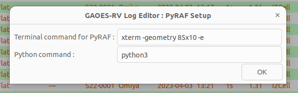
"Python command" is a python command required to start a python script for PyRAF such as "splot.py". If you needpython3 splot.py
when starting "splot.py" under the Shared directory, enter "python3". If you can start it onlysplot.py
in your command line, please leave it as a blank.
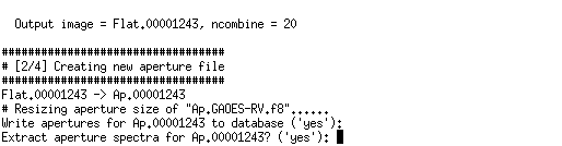
- Make Flat and Apeture
Flat and Aperture reference are created simultaneously from flat data.
When creating them for the first time, "Ap.GAOES-RV.f8.fits" under GAOES-RV_ql/ (automatically copied to your work directory) is used as a reference to recreate Aperture.
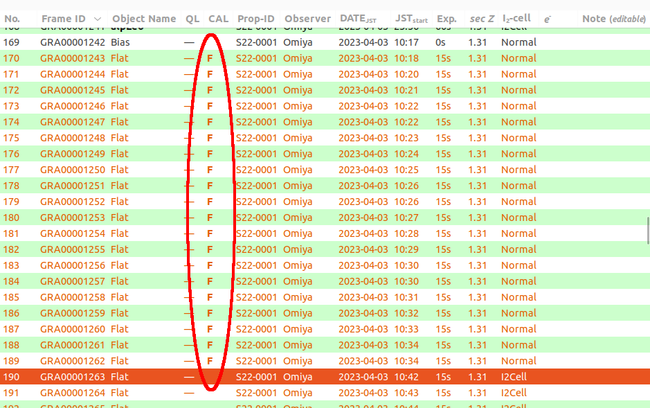
Select multiple flat frames as shown below and press the "Flat" button.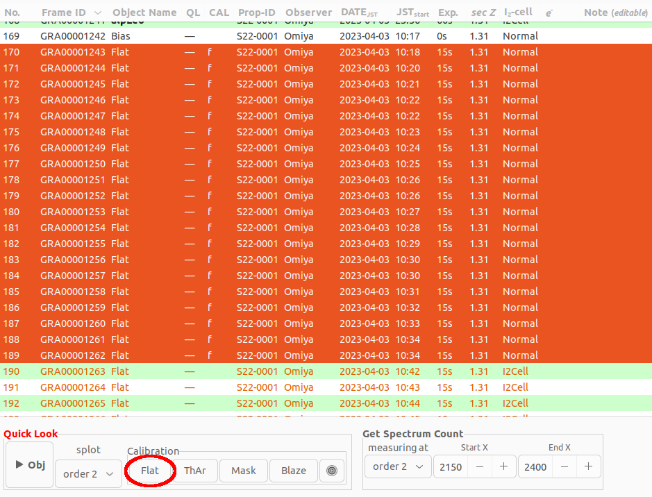
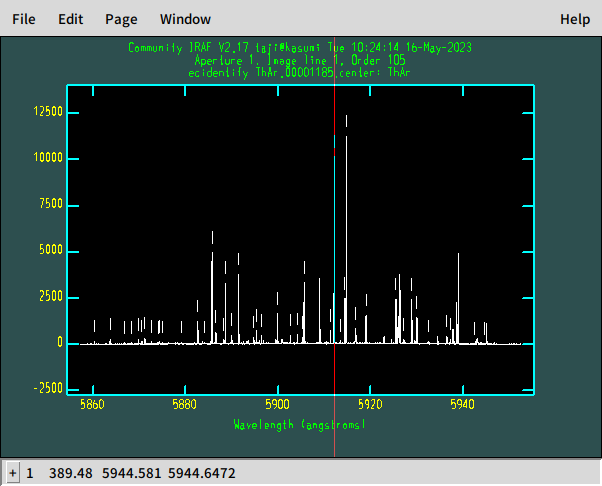
- Make Comparison
When creating for the first time, wavelength calibration data will be created using the reference to "ThAr.GAOES-RV.f8.center.fits" under GAOES-RV_ql/ (automatically copied to your work directory).
Select the ThAr frame you want to use as a wavelength calibration comparison in the table and press the "ThAr" button.
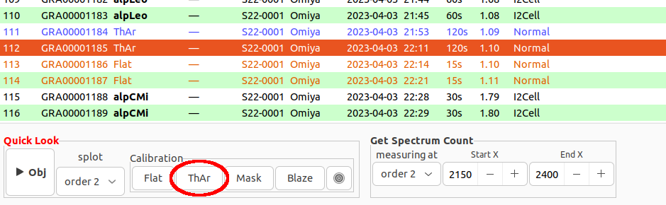
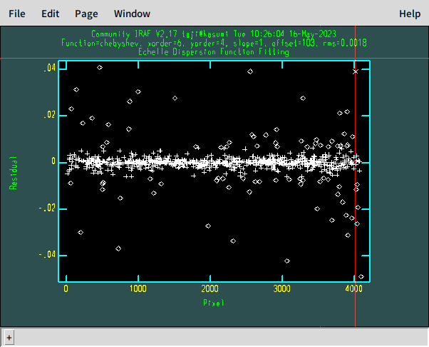
If the wavelength calibration data is created normally, a "C" mark will appear in the CAL column of the table.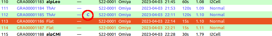
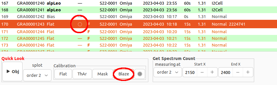
- Make Blaze function
Create a blaze function by performing a continuous light fit on the analyzed flat as well as object frames. This prcoess is required to make full 1D spectrum of objects (connecting each order of the echelle).
First, select one frame of flat and press the "Obj" button to analyze it.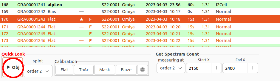
Please refer to here for details and operation.
- Make Mask (not necessary in usual
As with "Blaze", you can also create a mask for the analyzed flat using the "Mask" button.
Basically, you can leave "Mask.GAOES-RV.ocs_ecfw.fits" which is automatically copied under GAOES-RV_ql/, we won′t explain it here.
- Check CAL setting
You can check the current set CAL frame by pressing the gear mark button next to "Blaze" in the lower "Calibration" section. "Aperture", "Flat", "Wavelength reference", etc. are automatically set when each is successfully created. If you want to change it, you can change it with the button on the right of each frame.
In particular, if you want to recreate "Flat" or "ThAr" from the same frames, set the default file "Flat(ThAr).GAOES-RV..." once in this window and then create it again. (The database is deleted once to avoid overwriting, if you try to recreate a new one.)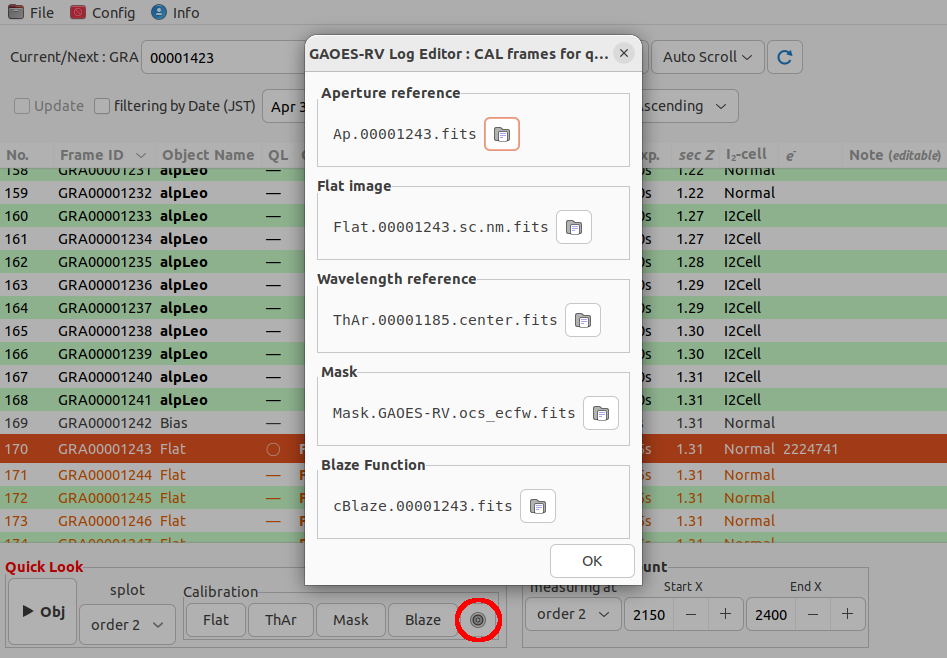
- Object analysis
After preparing CAL as above (if not prepared, reference below GAOES-RV_ql/ will be used), select a object frame, and press the "Obj" button to analyze it.
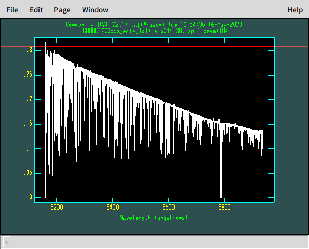
You can select the order of echelle or the full 1D spectrum (1D spec) to display in the "splot" task.
Also, in the "Get Spectrum Count" section, you can specify which pixels of which order for automatic measurement of the spectrum count.
You can also select multiple object frames for batch processing. Spectral plotting is skipped during batch processing.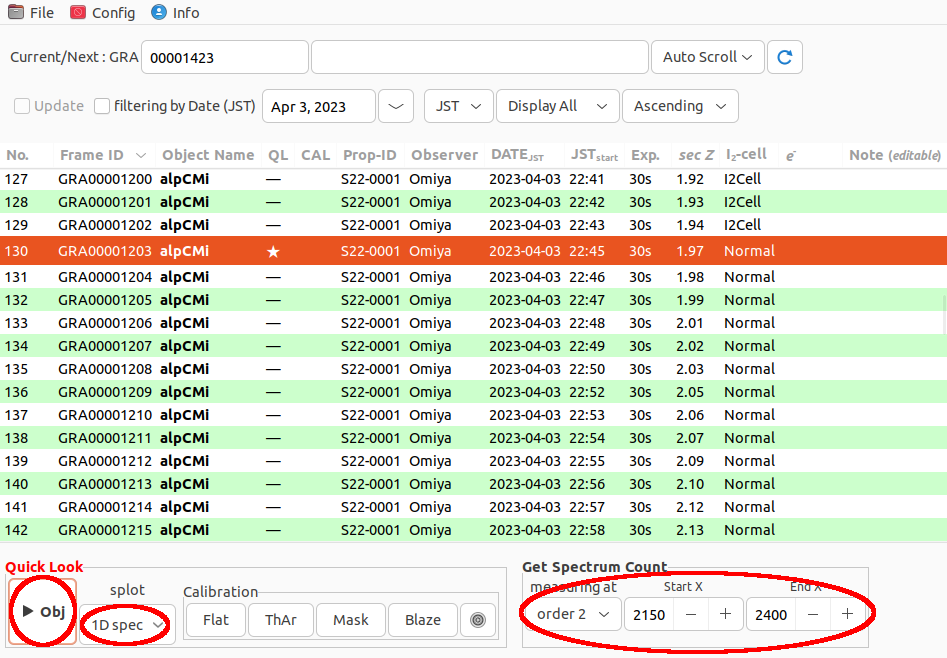
When the analysis is completed, the QL column of the table is marked with a circle, and the approximate count (number of photons) is entered in the e- column.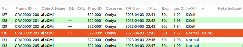
- Save Observation Log
The log can be output to a CSV file with File → Save Log in the menu. - Make Flat and Apeture